5. Conditionals

Programs get really interesting when we can test conditions and change the program behaviour depending on the outcome of the tests. That’s what this chapter is about.

5.1. Boolean values and expressions

A Boolean value is either true or false. It is named after the British mathematician, George Boole, who first formulated Boolean algebra — some rules for reasoning about and combining these values. This is the basis of all modern computer logic.

In Python, the two Boolean values are True and False (the capitalization must be exactly as shown), and the Python type is bool.

>>> type(True)
<class 'bool'>
>>> type(true)
Traceback (most recent call last):
  File "<interactive input>", line 1, in <module>
NameError: name 'true' is not defined

A Boolean expression is an expression that evaluates to produce a result which is a Boolean value. For example, the operator == tests if two values are equal. It produces (or yields) a Boolean value:

>>> 5 == (3 + 2)   # Is five equal 5 to the result of 3 + 2?
True
>>> 5 == 6
False
>>> j = "hel"
>>> j + "lo" == "hello"
True

In the first statement, the two operands evaluate to equal values, so the expression evaluates to True; in the second statement, 5 is not equal to 6, so we get False.

The == operator is one of six common comparison operators which all produce a bool result; here are all six:

x == y               # Produce True if ... x is equal to y
x != y               # ... x is not equal to y
x > y                # ... x is greater than y
x < y                # ... x is less than y
x >= y               # ... x is greater than or equal to y
x <= y               # ... x is less than or equal to y

Although these operations are probably familiar, the Python symbols are different from the mathematical symbols. A common error is to use a single equal sign (=) instead of a double equal sign (==). Remember that = is an assignment operator and == is a comparison operator. Also, there is no such thing as =< or =>.

Like any other types we’ve seen so far, Boolean values can be assigned to variables, printed, etc.

>>> age = 18
>>> old_enough_to_get_driving_licence = age >= 17
>>> print(old_enough_to_get_driving_licence)
True
>>> type(old_enough_to_get_driving_licence)
<class 'bool'>

5.2. Logical operators

There are three logical operators, and, or, and not, that allow us to build more complex Boolean expressions from simpler Boolean expressions. The semantics (meaning) of these operators is similar to their meaning in English. For example, x > 0 and x < 10 produces True only if x is greater than 0 and at the same time, x is less than 10.

n % 2 == 0 or n % 3 == 0 is True if either of the conditions is True, that is, if the number n is divisible by 2 or it is divisible by 3. (What do you think happens if n is divisible by both 2 and by 3 at the same time? Will the expression yield True or False? Try it in your Python interpreter.)

Finally, the not operator negates a Boolean value, so not (x > y) is True if (x > y) is False, that is, if x is less than or equal to y.

The expression on the left of the or operator is evaluated first: if the result is True, Python does not (and need not) evaluate the expression on the right — this is called short-circuit evaluation. Similarly, for the and operator, if the expression on the left yields False, Python does not evaluate the expression on the right.

So there are no unnecessary evaluations.

5.3. Truth Tables

A truth table is a small table that allows us to list all the possible inputs, and to give the results for the logical operators. Because the and and or operators each have two operands, there are only four rows in a truth table that describes the semantics of and.

a	b	a and b
False	False	False
False	True	False
True	False	False
True	True	True

In a Truth Table, we sometimes use T and F as shorthand for the two Boolean values: here is the truth table describing or:

a	b	a or b
F	F	F
F	T	T
T	F	T
T	T	T

The third logical operator, not, only takes a single operand, so its truth table only has two rows:

a	not a
F	T
T	F

5.4. Simplifying Boolean Expressions

A set of rules for simplifying and rearranging expressions is called an algebra. For example, we are all familiar with school algebra rules, such as:

n * 0 == 0

Here we see a different algebra — the Boolean algebra — which provides rules for working with Boolean values.

First, the and operator:

x and False == False
False and x == False
y and x == x and y
x and True == x
True and x == x
x and x == x

Here are some corresponding rules for the or operator:

x or False == x
False or x == x
y or x == x or y
x or True == True
True or x == True
x or x == x

Two not operators cancel each other:

not (not x) == x

5.5. Conditional execution

In order to write useful programs, we almost always need the ability to check conditions and change the behavior of the program accordingly. Conditional statements give us this ability. The simplest form is the if statement:

if x % 2 == 0:
    print(x, " is even.")
    print("Did you know that 2 is the only even number that is prime?")
else:
    print(x, " is odd.")
    print("Did you know that multiplying two odd numbers " +
                                         "always gives an odd result?")

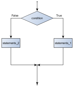
The Boolean expression after the if statement is called the condition. If it is true, then all the indented statements get executed. If not, then all the statements indented under the else clause get executed.

Flowchart of an if statement with an else clause

The syntax for an if statement looks like this:

if BOOLEAN EXPRESSION:
    STATEMENTS_1        # Executed if condition evaluates to True
else:
    STATEMENTS_2        # Executed if condition evaluates to False

As with the function definition from the last chapter and other compound statements like for, the if statement consists of a header line and a body. The header line begins with the keyword if followed by a Boolean expression and ends with a colon (:).

The indented statements that follow are called a block. The first unindented statement marks the end of the block.

Each of the statements inside the first block of statements are executed in order if the Boolean expression evaluates to True. The entire first block of statements is skipped if the Boolean expression evaluates to False, and instead all the statements indented under the else clause are executed.

There is no limit on the number of statements that can appear under the two clauses of an if statement, but there has to be at least one statement in each block. Occasionally, it is useful to have a section with no statements (usually as a place keeper, or scaffolding, for code we haven’t written yet). In that case, we can use the pass statement, which does nothing except act as a placeholder.

if True:          # This is always True,
    pass          #   so this is always executed, but it does nothing
else:
    pass

5.6. Omitting the else clause

Flowchart of an if statement with no else clause

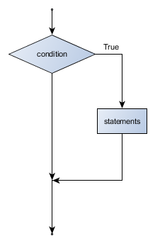
Another form of the if statement is one in which the else clause is omitted entirely. In this case, when the condition evaluates to True, the statements are executed, otherwise the flow of execution continues to the statement after the if.

if x < 0:
    print("The negative number ",  x, " is not valid here.")
    x = 42
    print("I've decided to use the number 42 instead.")

print("The square root of ", x, "is", math.sqrt(x))

In this case, the print function that outputs the square root is the one after the if — not because we left a blank line, but because of the way the code is indented. Note too that the function call math.sqrt(x) will give an error unless we have an import math statement, usually placed near the top of our script.

Python terminology

Python documentation sometimes uses the term suite of statements to mean what we have called a block here. They mean the same thing, and since most other languages and computer scientists use the word block, we’ll stick with that.

Notice too that else is not a statement. The if statement has two clauses, one of which is the (optional) else clause.

5.7. Chained conditionals

Sometimes there are more than two possibilities and we need more than two branches. One way to express a computation like that is a chained conditional:

if x < y:
    STATEMENTS_A
elif x > y:
    STATEMENTS_B
else:
    STATEMENTS_C

Flowchart of this chained conditional

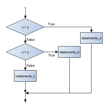
elif is an abbreviation of else if. Again, exactly one branch will be executed. There is no limit of the number of elif statements but only a single (and optional) final else statement is allowed and it must be the last branch in the statement:

if choice == "a":
    function_one()
elif choice == "b":
    function_two()
elif choice == "c":
    function_three()
else:
    print("Invalid choice.")

Each condition is checked in order. If the first is false, the next is checked, and so on. If one of them is true, the corresponding branch executes, and the statement ends. Even if more than one condition is true, only the first true branch executes.

5.8. Nested conditionals

One conditional can also be nested within another. (It is the same theme of composibility, again!) We could have written the previous example as follows:

Flowchart of this nested conditional

if x < y:
    STATEMENTS_A
else:
    if x > y:
        STATEMENTS_B
    else:
        STATEMENTS_C

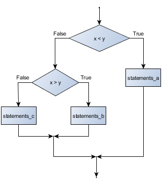
The outer conditional contains two branches. The second branch contains another if statement, which has two branches of its own. Those two branches could contain conditional statements as well.

Although the indentation of the statements makes the structure apparent, nested conditionals very quickly become difficult to read. In general, it is a good idea to avoid them when we can.

Logical operators often provide a way to simplify nested conditional statements. For example, we can rewrite the following code using a single conditional:

if 0 < x:            # Assume x is an int here
    if x < 10:
        print("x is a positive single digit.")

The print function is called only if we make it past both the conditionals, so instead of the above which uses two if statements each with a simple condition, we could make a more complex condition using the and operator. Now we only need a single if statement:

if 0 < x and x < 10:
    print("x is a positive single digit.")

5.9. The return statement

The return statement, with or without a value, depending on whether the function is fruitful or void, allows us to terminate the execution of a function before (or when) we reach the end. One reason to use an early return is if we detect an error condition:

def print_square_root(x):
    if x <= 0:
        print("Positive numbers only, please.")
        return

    result = x**0.5
    print("The square root of", x, "is", result)

The function print_square_root has a parameter named x. The first thing it does is check whether x is less than or equal to 0, in which case it displays an error message and then uses return to exit the function. The flow of execution immediately returns to the caller, and the remaining lines of the function are not executed.

5.10. Logical opposites

Each of the six relational operators has a logical opposite: for example, suppose we can get a driving licence when our age is greater or equal to 17, we can not get the driving licence when we are less than 17.

Notice that the opposite of >= is <.

operator	logical opposite
==	!=
!=	==
<	>=
<=	>
>	<=
>=	<

Understanding these logical opposites allows us to sometimes get rid of not operators. not operators are often quite difficult to read in computer code, and our intentions will usually be clearer if we can eliminate them.

For example, if we wrote this Python:

if not (age >= 17):
    print("Hey, you're too young to get a driving licence!")

it would probably be clearer to use the simplification laws, and to write instead:

if age < 17:
    print("Hey, you're too young to get a driving licence!")

Two powerful simplification laws (called de Morgan’s laws) that are often helpful when dealing with complicated Boolean expressions are:

not (x and y)  ==  (not x) or (not y)
not (x or y)   ==  (not x) and (not y)

For example, suppose we can slay the dragon only if our magic lightsabre sword is charged to 90% or higher, and we have 100 or more energy units in our protective shield. We find this fragment of Python code in the game:

if not ((sword_charge >= 0.90) and (shield_energy >= 100)):
    print("Your attack has no effect, the dragon fries you to a crisp!")
else:
    print("The dragon crumples in a heap. You rescue the gorgeous princess!")

de Morgan’s laws together with the logical opposites would let us rework the condition in a (perhaps) easier to understand way like this:

if (sword_charge < 0.90) or (shield_energy < 100):
    print("Your attack has no effect, the dragon fries you to a crisp!")
else:
    print("The dragon crumples in a heap. You rescue the gorgeous princess!")

We could also get rid of the not by swapping around the then and else parts of the conditional. So here is a third version, also equivalent:

if (sword_charge >= 0.90) and (shield_energy >= 100):
    print("The dragon crumples in a heap. You rescue the gorgeous princess!")
else:
    print("Your attack has no effect, the dragon fries you to a crisp!")

This version is probably the best of the three, because it very closely matches the initial English statement. Clarity of our code (for other humans), and making it easy to see that the code does what was expected should always be a high priority.

As our programming skills develop we’ll find we have more than one way to solve any problem. So good programs are designed. We make choices that favour clarity, simplicity, and elegance. The job title software architect says a lot about what we do — we are architects who engineer our products to balance beauty, functionality, simplicity and clarity in our creations.

Tip

Once our program works, we should play around a bit trying to polish it up. Write good comments. Think about whether the code would be clearer with different variable names. Could we have done it more elegantly? Should we rather use a function? Can we simplify the conditionals?

We think of our code as our creation, our work of art! We make it great.

5.11. Type conversion

We’ve had a first look at this in an earlier chapter. Seeing it again won’t hurt!

Many Python types come with a built-in function that attempts to convert values of another type into its own type. The int function, for example, takes any value and converts it to an integer, if possible, or complains otherwise:

>>> int("32")
32
>>> int("Hello")
ValueError: invalid literal for int() with base 10: 'Hello'

int can also convert floating-point values to integers, but remember that it truncates the fractional part:

>>> int(-2.3)
-2
>>> int(3.99999)
3
>>> int("42")
42
>>> int(1.0)
1

The float function converts integers and strings to floating-point numbers:

>>> float(32)
32.0
>>> float("3.14159")
3.14159
>>> float(1)
1.0

It may seem odd that Python distinguishes the integer value 1 from the floating-point value 1.0. They may represent the same number, but they belong to different types. The reason is that they are represented differently inside the computer.

The str function converts any argument given to it to type string:

>>> str(32)
'32'
>>> str(3.14149)
'3.14149'
>>> str(True)
'True'
>>> str(true)
Traceback (most recent call last):
  File "<interactive input>", line 1, in <module>
NameError: name 'true' is not defined

str will work with any value and convert it into a string. As mentioned earlier, True is Boolean value; true is just an ordinary variable name, and is not defined here, so we get an error.

5.12. A Turtle Bar Chart

The turtle has a lot more power than we’ve seen so far. The full documentation can be found at http://docs.python.org/py3k/library/turtle.html or within PyScripter, use Help and search for the turtle module.

Here are a couple of new tricks for our turtles:

• We can get a turtle to display text on the canvas at the turtle’s current position. The method to do that is alex.write("Hello").
• We can fill a shape (circle, semicircle, triangle, etc.) with a color. It is a two-step process. First we call the method alex.begin_fill(), then we draw the shape, then we call alex.end_fill().
• We’ve previously set the color of our turtle — we can now also set its fill color, which need not be the same as the turtle and the pen color. We use alex.color("blue","red") to set the turtle to draw in blue, and fill in red.

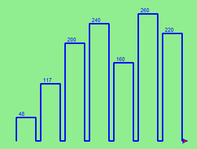
Ok, so can we get tess to draw a bar chart? Let us start with some data to be charted,

xs = [48, 117, 200, 240, 160, 260, 220]

Corresponding to each data measurement, we’ll draw a simple rectangle of that height, with a fixed width.

def draw_bar(t, height):
    """ Get turtle t to draw one bar, of height. """
    t.left(90)
    t.forward(height)     # Draw up the left side
    t.right(90)
    t.forward(40)         # Width of bar, along the top
    t.right(90)
    t.forward(height)     # And down again!
    t.left(90)            # Put the turtle facing the way we found it.
    t.forward(10)         # Leave small gap after each bar

...
for v in xs:              # Assume xs and tess are ready
    draw_bar(tess, v)

Ok, not fantasically impressive, but it is a nice start! The important thing here was the mental chunking, or how we broke the problem into smaller pieces. Our chunk is to draw one bar, and we wrote a function to do that. Then, for the whole chart, we repeatedly called our function.

Next, at the top of each bar, we’ll print the value of the data. We’ll do this in the body of draw_bar, by adding t.write('  ' + str(height)) as the new third line of the body. We’ve put a little space in front of the number, and turned the number into a string. Without this extra space we tend to cramp our text awkwardly against the bar to the left. The result looks a lot better now:

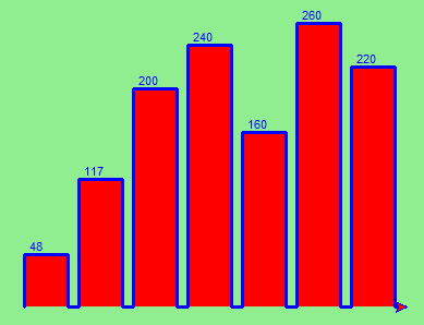
And now we’ll add two lines to fill each bar. Our final program now looks like this:

def draw_bar(t, height):
    """ Get turtle t to draw one bar, of height. """
    t.begin_fill()           # Added this line
    t.left(90)
    t.forward(height)
    t.write("  "+ str(height))
    t.right(90)
    t.forward(40)
    t.right(90)
    t.forward(height)
    t.left(90)
    t.end_fill()             # Added this line
    t.forward(10)

wn = turtle.Screen()         # Set up the window and its attributes
wn.bgcolor("lightgreen")

tess = turtle.Turtle()       # Create tess and set some attributes
tess.color("blue", "red")
tess.pensize(3)

xs = [48,117,200,240,160,260,220]

for a in xs:
    draw_bar(tess, a)

wn.mainloop()

It produces the following, which is more satisfying:

Mmm. Perhaps the bars should not be joined to each other at the bottom. We’ll need to pick up the pen while making the gap between the bars. We’ll leave that as an exercise for you!

5.13. Glossary

block

A group of consecutive statements with the same indentation.

body

The block of statements in a compound statement that follows the header.

Boolean algebra

Some rules for rearranging and reasoning about Boolean expressions.

Boolean expression

An expression that is either true or false.

Boolean value

There are exactly two Boolean values: True and False. Boolean values result when a Boolean expression is evaluated by the Python interepreter. They have type bool.

branch

One of the possible paths of the flow of execution determined by conditional execution.

chained conditional

A conditional branch with more than two possible flows of execution. In Python chained conditionals are written with if ... elif ... else statements.

comparison operator

One of the six operators that compares two values: ==, !=, >, <, >=, and <=.

condition

The Boolean expression in a conditional statement that determines which branch is executed.

conditional statement

A statement that controls the flow of execution depending on some condition. In Python the keywords if, elif, and else are used for conditional statements.

logical operator

One of the operators that combines Boolean expressions: and, or, and not.

nesting

One program structure within another, such as a conditional statement inside a branch of another conditional statement.

prompt

A visual cue that tells the user that the system is ready to accept input data.

truth table

A concise table of Boolean values that can describe the semantics of an operator.

type conversion

An explicit function call that takes a value of one type and computes a corresponding value of another type.

wrapping code in a function

The process of adding a function header and parameters to a sequence of program statements is often refered to as “wrapping the code in a function”. This process is very useful whenever the program statements in question are going to be used multiple times. It is even more useful when it allows the programmer to express their mental chunking, and how they’ve broken a complex problem into pieces.

5.14. Exercises

1. Assume the days of the week are numbered 0,1,2,3,4,5,6 from Sunday to Saturday. Write a function which is given the day number, and it returns the day name (a string).

2. You go on a wonderful holiday (perhaps to jail, if you don’t like happy exercises) leaving on day number 3 (a Wednesday). You return home after 137 sleeps. Write a general version of the program which asks for the starting day number, and the length of your stay, and it will tell you the name of day of the week you will return on.

3. Give the logical opposites of these conditions

   1. a > b
   2. a >= b
   3. a >= 18  and  day == 3
   4. a >= 18  and  day != 3

4. What do these expressions evaluate to?

   1. 3 == 3
   2. 3 != 3
   3. 3 >= 4
   4. not (3 < 4)

5. Complete this truth table:

   p	q	r	(not (p and q)) or r
   F	F	F	?
   F	F	T	?
   F	T	F	?
   F	T	T	?
   T	F	F	?
   T	F	T	?
   T	T	F	?
   T	T	T	?

6. Write a function which is given an exam mark, and it returns a string — the grade for that mark — according to this scheme:

   Mark	Grade
   >= 75	First
   [70-75)	Upper Second
   [60-70)	Second
   [50-60)	Third
   [45-50)	F1 Supp
   [40-45)	F2
   < 40	F3

   The square and round brackets denote closed and open intervals. A closed interval includes the number, and open interval excludes it. So 39.99999 gets grade F3, but 40 gets grade F2. Assume

   xs = [83, 75, 74.9, 70, 69.9, 65, 60, 59.9, 55, 50,
                        49.9, 45, 44.9, 40, 39.9, 2, 0]
   

   Test your function by printing the mark and the grade for all the elements in this list.

7. Modify the turtle bar chart program so that the pen is up for the small gaps between each bar.

8. Modify the turtle bar chart program so that the bar for any value of 200 or more is filled with red, values between [100 and 200) are filled with yellow, and bars representing values less than 100 are filled with green.

9. In the turtle bar chart program, what do you expect to happen if one or more of the data values in the list is negative? Try it out. Change the program so that when it prints the text value for the negative bars, it puts the text below the bottom of the bar.

10. Write a function find_hypot which, given the length of two sides of a right-angled triangle, returns the length of the hypotenuse. (Hint: x ** 0.5 will return the square root.)

11. Write a function is_rightangled which, given the length of three sides of a triangle, will determine whether the triangle is right-angled. Assume that the third argument to the function is always the longest side. It will return True if the triangle is right-angled, or False otherwise.

    Hint: Floating point arithmetic is not always exactly accurate, so it is not safe to test floating point numbers for equality. If a good programmer wants to know whether x is equal or close enough to y, they would probably code it up as:

    if  abs(x-y) < 0.000001:    # If x is approximately equal to y
        ...
    

12. Extend the above program so that the sides can be given to the function in any order.

13. If you’re intrigued by why floating point arithmetic is sometimes inaccurate, on a piece of paper, divide 10 by 3 and write down the decimal result. You’ll find it does not terminate, so you’ll need an infinitely long sheet of paper. The representation of numbers in computer memory or on your calculator has similar problems: memory is finite, and some digits may have to be discarded. So small inaccuracies creep in. Try this script:

  import math
  a = math.sqrt(2.0)
  print(a, a*a)
  print(a*a == 2.0)